DeepSeek's mHC: When Residual Connections Explode
- Method
- A 10M-parameter GPT-2 on TinyShakespeare for 5,000 steps, unconstrained Hyper-Connections against the Sinkhorn-constrained version as separate training runs: three seeds at depth 24, and one run per depth from 6 to 24 layers at a constant parameter budget. Amax, the maximum row or column absolute sum of the mixing matrix, is the measure.
- Result
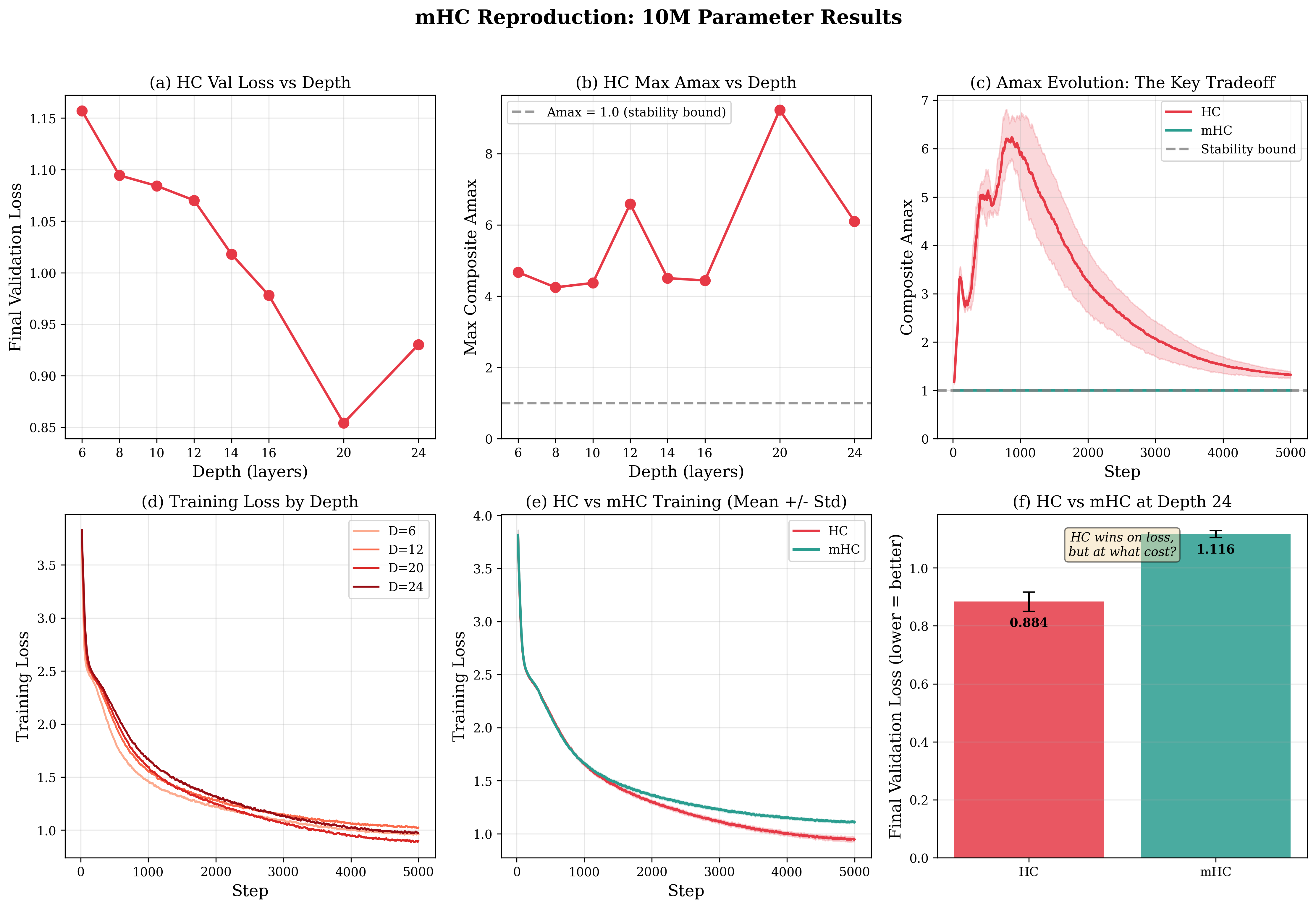
- Reproduced the 9× signal amplification in DeepSeek's Hyper-Connections at 10M parameters, and the fix: Sinkhorn-Knopp normalisation of the mixing matrices.
- Could not detect
- Three seeds, reported as a mean and standard deviation with no interval claimed beyond them. One seed per depth, so the depth sweep's scatter cannot be separated from seed noise and no trend is fitted. Separate trainings: no paired test and no minimum detectable effect apply.
- Artifacts
- code
Every transformer in use today carries the same residual connection design from 2016. GPT-5, Claude, Llama, Gemini: under the hood they all do , one stream of information through the network, each layer adding to it. DeepSeek asked what happens if you make that stream wider.
The setup
The standard residual connection is the one every modern transformer uses:
The input passes through unchanged and the layer’s output is added to it. That clean path backward is why transformers can be hundreds of layers deep, and it hasn’t changed since 2016.
Hyper-Connections widen that to n parallel streams with learnable mixing matrices:
Compared to standard residual:
Three matrices control how information flows:
- H_res: How streams mix in the residual path (the crossings above)
- H_pre: How streams combine before entering the layer
- H_post: How the layer’s output distributes back to streams
That’s more expressive, for almost no extra compute, and in theory it should perform better. The catch is that the mixing matrices are unconstrained. They can amplify a signal, not just route it.
The explosion
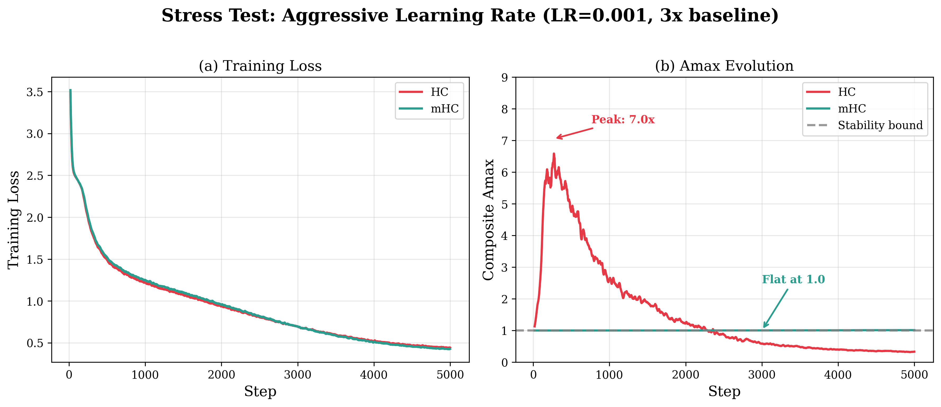
Under aggressive learning rates, Hyper-Connection (HC) signal amplification in my reproduction hit 7x before eventually collapsing. Amax (the maximum of row and column absolute sums) measures how much a matrix can amplify signals.
At 10M parameters that’s survivable. DeepSeek saw this at 27B:
“The Amax Gain Magnitude yields extreme values with peaks of 3000”
Three thousand times. At 27B parameters unconstrained HC doesn’t drift, it blows up, and the 9.2× I saw at 10M is the same thing early. Small amplifications compound layer over layer.
The fix: constrain the manifold
DeepSeek’s fix is to constrain the mixing matrices to be doubly stochastic.
A doubly stochastic matrix has:
- All non-negative entries
- Rows sum to 1
- Columns sum to 1
So the mixing operation can only take weighted averages of streams. It can route, shuffle and blend, and it can’t amplify. The way to get there is the Sinkhorn-Knopp algorithm.
The algorithm is short:
- Start with any matrix (the raw learned weights)
- Exponentiate to make all entries positive:
- Normalize rows so each row sums to 1
- Normalize columns so each column sums to 1
- Repeat steps 3-4 until convergence
Alternate row and column normalisation; twenty iterations is enough.
This procedure is differentiable. Gradients flow back through all twenty iterations. The network learns the raw weights , and Sinkhorn ensures the actual mixing matrix is always doubly stochastic.
When I first saw this it felt like cheating: you’re not learning stability, you’re forcing it. I’ve come round to it. Some properties shouldn’t be learned, they should be guaranteed.
Strictly, only the recursive matrix H_res needs the full Sinkhorn treatment, since it’s the one compounding layer over layer. The input and output mixers, H_pre and H_post, are just bounded with a sigmoid, so the Sinkhorn cost is paid only where it matters.
The results
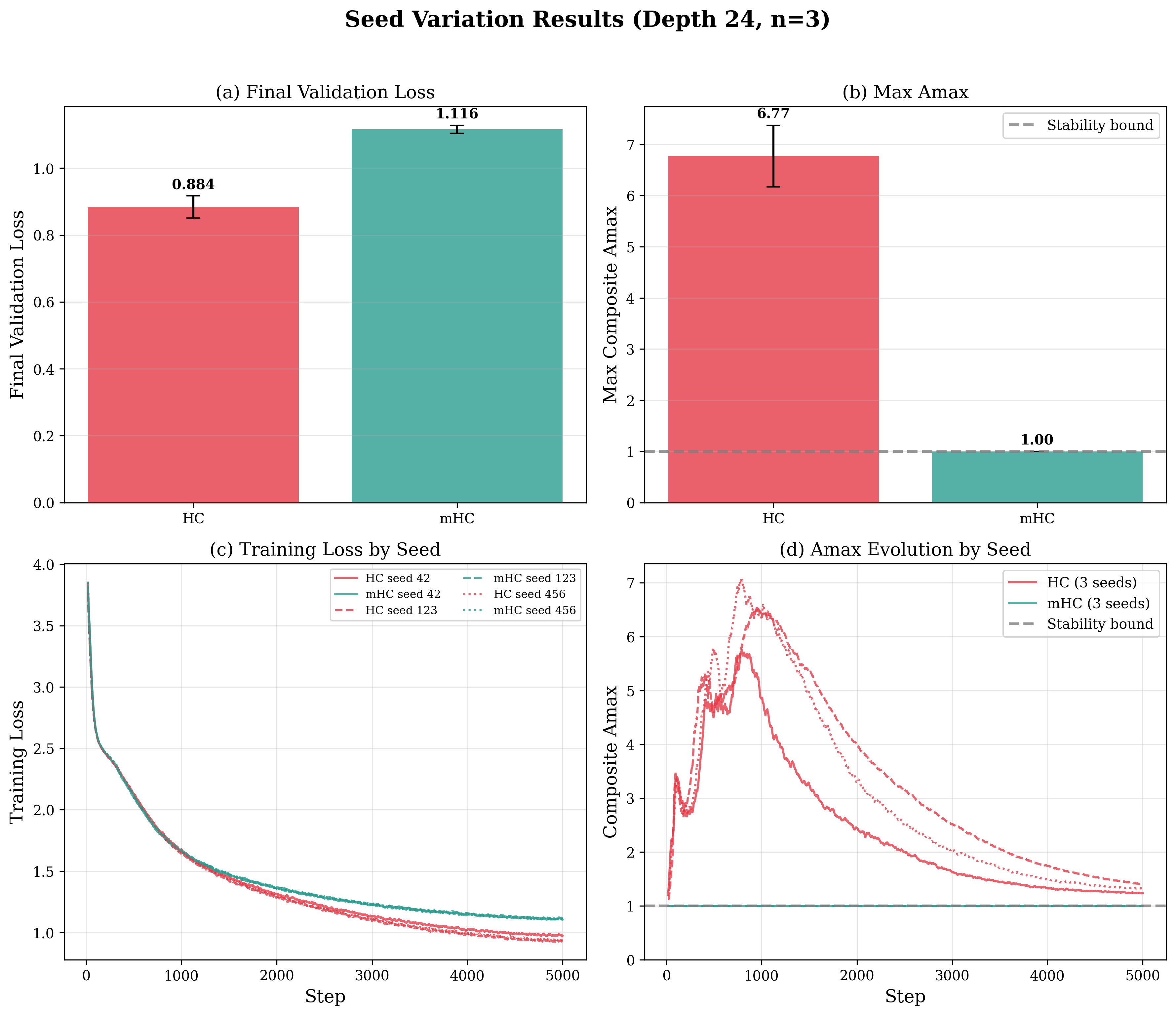
Seed variation, depth 24, three seeds
| Model | Val Loss (mean ± std) | Max Amax (mean ± std) |
|---|---|---|
| HC | 0.884 ± 0.033 | 6.77 ± 0.60 |
| mHC | 1.116 ± 0.012 | 1.00 ± 0.00 |
HC wins on raw loss, 0.88 against 1.12. At 10M parameters the constraint reads as a tax on expressivity. The variance is the other half of the story: HC’s loss varies about three times as much across seeds (±0.033 against ±0.012), and its peak Amax swings from 6.1 to 7.6 depending on the seed, while mHC is 1.00 in every run. At this scale the instability is survivable and HC still wins. At 27B, per DeepSeek, 6 to 7× becomes 3000×, and the tax is what keeps the model out of NaN.
Depth scaling
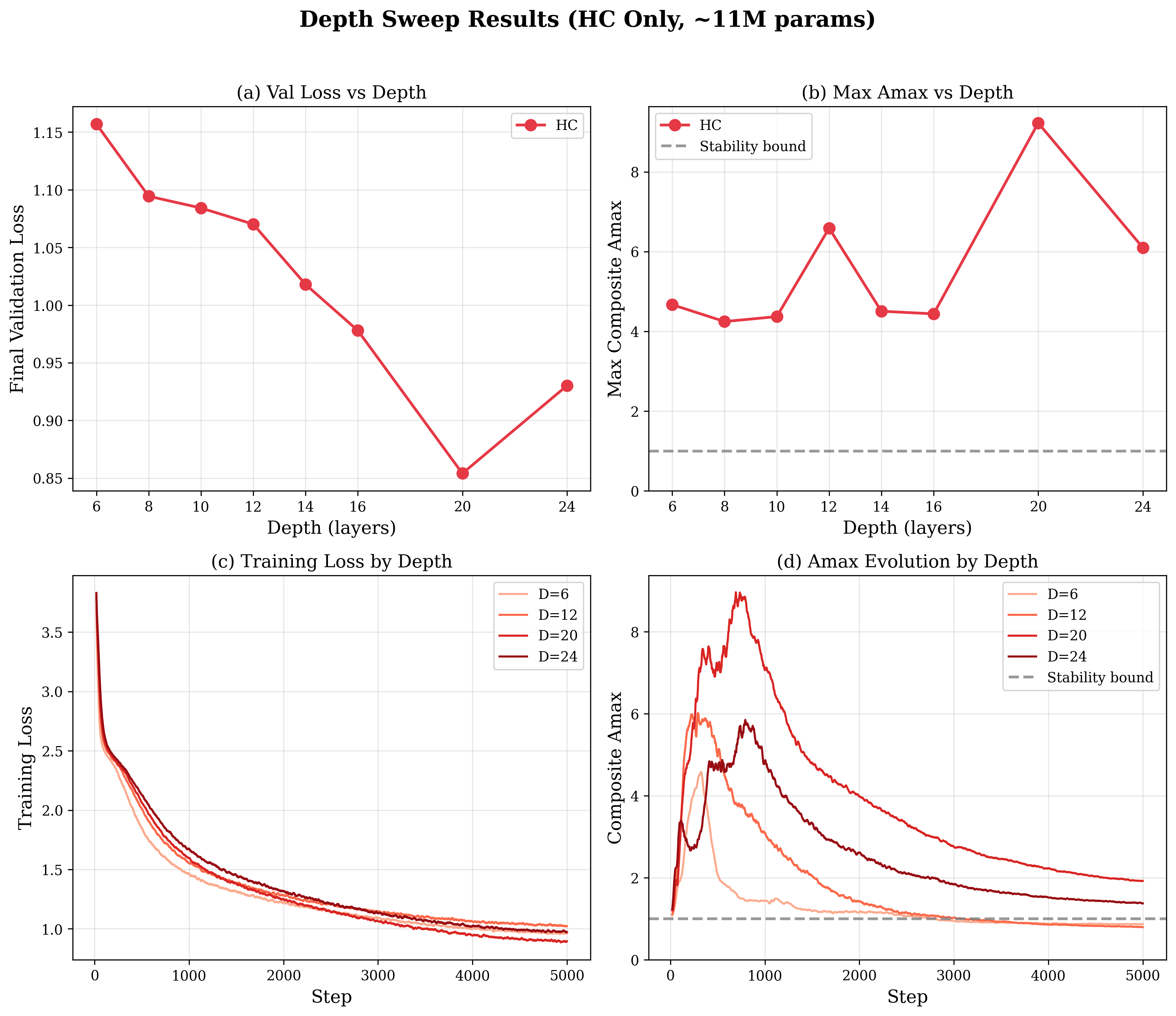
I also swept depth from 6 to 24 layers at a constant budget of about 11M parameters. Loss improves with depth up to 20 (0.85) and regresses at 24 (0.93), where the width has shrunk to 192. Peak Amax has no clean relationship with depth at all: 9.2× at depth 20, 6.6× at 12, 4.3× at 8, and with one seed per depth I can’t separate that scatter from seed noise.
Experiment details
Dataset: TinyShakespeare (~1M chars, character-level) Model: GPT-2 architecture, ~10M parameters Training: 5000 steps, AdamW (β1=0.9, β2=0.95), weight decay 0.1, cosine LR decay Hardware: Apple M-series (MPS)
Depth sweep: 8 configurations (6-24 layers), width adjusted to maintain ~11M params Seed variation: 3 seeds (42, 123, 456) at depth 24
Why this matters
The way I’ve come to think about it: a residual connection is a conservation law. The identity path keeps signal magnitude where it was, and that’s what lets the network be deep. He et al. introduced it in 2016 so signals wouldn’t die on the way back; ten years on, Hyper-Connections produced the opposite problem, signals growing on the way forward. HC breaks the conservation. mHC puts it back, not by returning to the identity but by finding a wider space of mixings that still conserve.
Every residual connection is a conservation law. mHC enforces it.
Takeaways
-
The stream persistence bug humbled me. My first implementation looked right. The equations matched the paper. The code ran. But I was projecting the output back to a single stream and re-expanding it at each layer, killing the parallel architecture. The “hyper” part of Hyper-Connections wasn’t actually doing anything. Three separate audits said “looks correct.” The bug was architectural, not mathematical. I only caught it by asking: “Wait, what shape is actually flowing between layers?”
-
The constraint is the point. The doubly stochastic projection doesn’t learn good behaviour, it makes bad behaviour impossible. My first reaction was that it’s a straitjacket. Then I watched HC hit 7× and understood why you’d want one.
-
Stable beats optimal. Standard residuals have lasted since 2016 because they’re stable, not because they’re the best possible choice. HC is more expressive and fragile. mHC sits between them: more expressive than a plain residual, with the stability guaranteed.
What’s next
This is Part 1 of a two-part series.
Part 1 (this post): Reproduce mHC at small scale to understand the mechanics.
- 10M parameters, TinyShakespeare dataset
- Constant parameter budget across depths
- Goal: Validate the core claim: HC explodes, mHC doesn’t
Part 2: Scale up to see real instability.
- 1.7B parameters on 8x H100s
- C4 dataset, fixed width (no bottleneck)
- Goal: Push toward the 3000x Amax regime
At 10M params, HC peaked at 9.2x amplification, chaotic but survivable. The paper saw 3000x at 27B. Part 2 shows what happens at scale: 10,924x.
Resources
Paper: Manifold-Constrained Hyper-Connections (arXiv 2512.24880)
Related: Deep Residual Learning (He et al., 2016)
Code: github.com/poisson-labs/mhc-repro
Part 2 is live. Follow @TayKolasinski for future posts.