10,924x: The Instability Bomb at 1.7B Scale

January 16, 2026

Method: Eighteen runs on C4: standard residual, unconstrained and Sinkhorn-constrained Hyper-Connections at depths 32 and 48, three seeds each, 5,000 steps in bf16 on an 8×H100 node, plus one run per configuration at three times the learning rate. Peak Amax per run is the measure, with loss and gradient norm alongside.
Result: Scaled the reproduction from 10M to 1.7B parameters: unconstrained Hyper-Connections reached 10,924× signal amplification; the Sinkhorn-constrained version held at 1.0.
Could not detect: Separate trainings, so no paired test and no minimum detectable effect apply; three seeds per cell, reported as a standard deviation. Three points, one of them another paper's architecture and recipe, do not make a scaling law, and whether the amplification eventually causes a failure is open: nothing crashed within 5,000 steps.
Artifacts: code · data · stress data

Part 2 of the mHC reproduction series. Part 1 showed the instability at 10M parameters. Now I scale up.

In Part 1 I trained a 10M parameter transformer on TinyShakespeare and watched Hyper-Connections reach 9.2× signal amplification. The DeepSeek paper reported 3000× at 27B, and I wanted to see how far I could get toward that number.

Is there a better feeling than the first SSH into fresh metal, GPUs unaware of the hours of abuse they’re about to endure?

Not really. I rented an 8×H100 node and put about thirteen hours of runs through it. Here’s what came out of it.

The scale jump

	Part 1	Part 2
Parameters	10M	1.7B - 2.5B
Dataset	TinyShakespeare (1MB)	C4 (300GB+)
Hardware	M4 MacBook	8x H100 SXM5
Max Amax	9.2x	10,924x

Ten thousand nine hundred and twenty-four times, well past the 3000× the paper reported.

The experiment

I ran 18 experiments across three architectures:

Residual: Standard x + F(x) baseline
HC: Hyper-Connections with unconstrained mixing matrices
mHC: Manifold Hyper-Connections with Sinkhorn projection

Each architecture at two depths (32 and 48 layers), three seeds each (42, 123, 456). All trained for 5000 steps on C4 with bf16 mixed precision.

The 32-layer models have 1.73B parameters while the 48-layer models have 2.54B.

The results

Six panels: training loss and signal amplification and gradient norm, at depth 32 and depth 48. The loss curves for all three architectures overlap; the unconstrained amplification curve climbs into the thousands while the constrained one is flat. — *Fig. 1* Eighteen runs on C4: three architectures (standard residual, unconstrained Hyper-Connections, Sinkhorn-constrained) at two depths (32 and 48 layers) and three seeds each, 5,000 steps, bf16, on an 8×H100 node. Loss panels: all three converge together, so the constraint costs nothing measurable here. Amax panels: unconstrained amplification climbs into the thousands and oscillates, while the constrained arm holds at 1.0. Colour separates the three architectures, not a verdict, and each is labelled. The runs are unpaired — separate trainings, not the same run measured twice — so no paired test and no minimum detectable effect apply anywhere in this post.

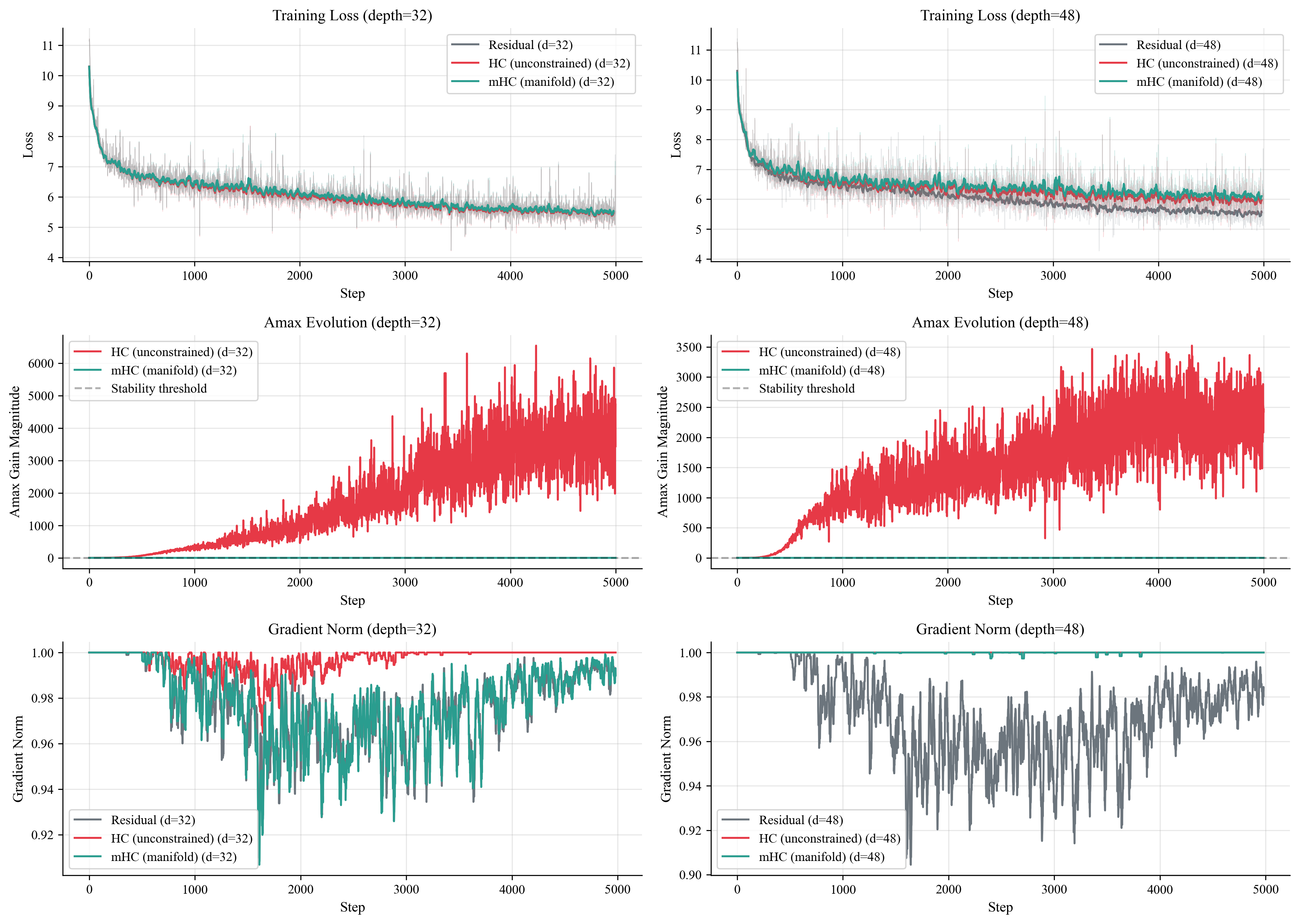
Loss: all three learn the same

All three converge to similar loss, about 5.4 to 6.0, and the curves overlap almost perfectly. HC doesn’t learn faster and mHC doesn’t learn slower. At this scale Sinkhorn was free, which I didn’t expect.

Amax

Amax, as in Part 1, is how much a mixing matrix can amplify a signal: 1.0 is neutral, higher is amplification.

hc_d32_s42 6,544.899× hc_d32_s123 11,919.215× hc_d32_s456 14,308.401× mhc_d32_s42 1.0000019× mhc_d32_s123 1.0000017× mhc_d32_s456 1.0000017×

Fig. 2Composite signal amplification against training step, log scale: three seeds of unconstrained Hyper-Connections against three of the Sinkhorn-constrained version, depth 32 on C4, 5,000 steps each. Purple and solid is the arm that diverges; green and dashed is the arm that holds, and each is named on the figure, so the distinction never rests on hue. The six runs are separate trainings rather than one run measured twice, so no paired test and no minimum detectable effect apply.

HC, unconstrained — solid mHC, Sinkhorn-constrained — dashed peak over all 5,000 stored steps

Peak amplification per run, taken over the full stored series before the downsample; the drawn curve keeps every 34th stored step, so a peak mark can sit above the highest point on its line. The three HC peaks average 10,924.172×, which is the number the post quotes. The three mHC runs never leave 1.0 — on this scale all three sit on the axis floor.

At depth 32, HC’s Amax climbs to between 6,500× and 14,300× depending on the seed, oscillating the whole way, while mHC sits at exactly 1.0. At depth 48 the pattern repeats: HC reaches about 3,500×, mHC stays at 1.0.

The numbers

Method	Depth	Final Loss	Max Amax
Residual	32	5.45 ± 0.04	N/A
HC	32	5.43 ± 0.03	10,924 ± 3,247
mHC	32	5.45 ± 0.03	1.00 ± 0.00
Residual	48	5.48 ± 0.04	N/A
HC	48	5.92 ± 0.19	3,721 ± 378
mHC	48	6.03 ± 0.20	1.00 ± 0.00

The variance is the thing to look at. HC at depth 32 peaks at 6,545, 11,919 and 14,308 across the three seeds. mHC is 1.00 in each run, with no variance at all.

The scaling law

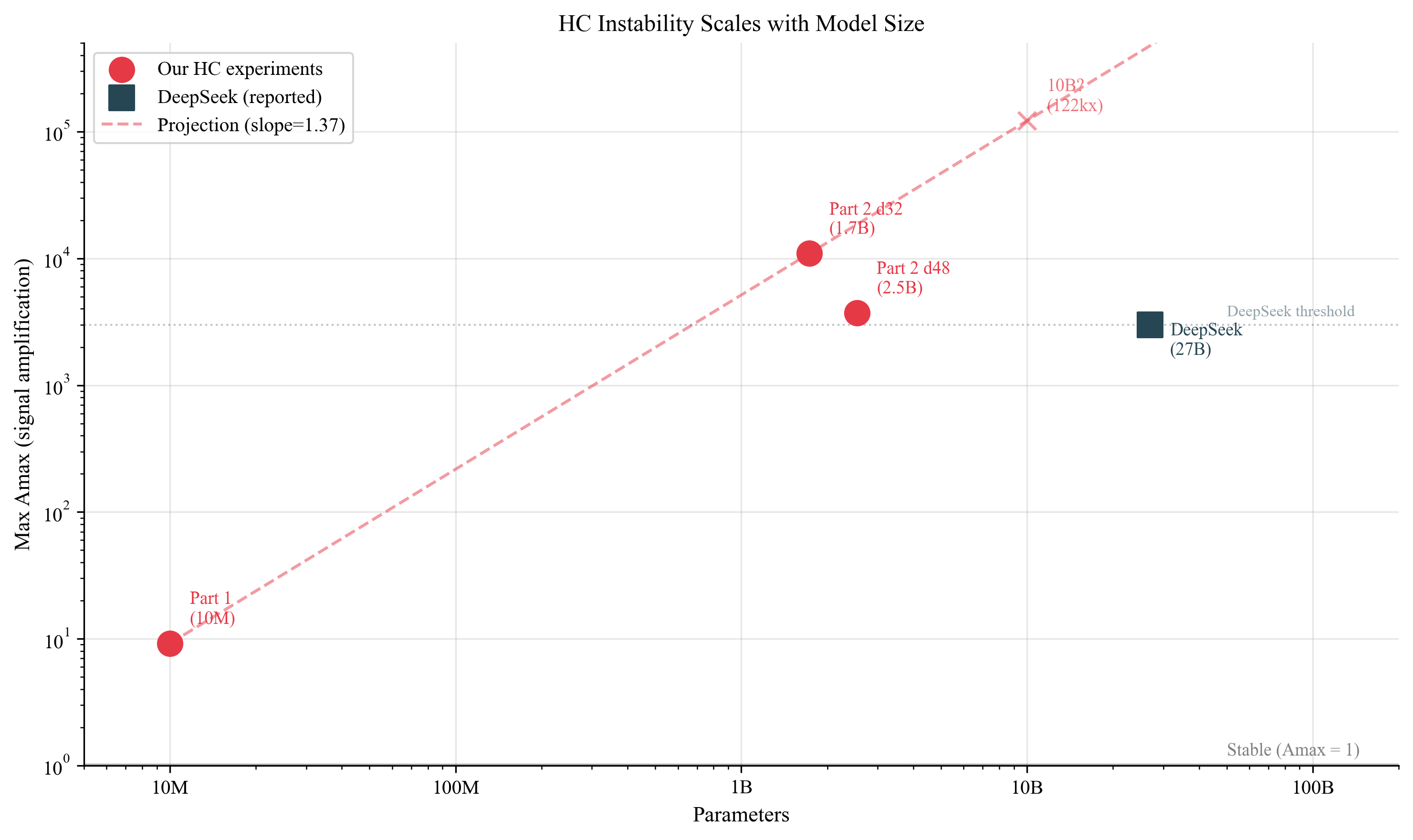
Log-log plot of peak signal amplification against parameter count, with three points: 10M, 1.7B, and a reported 27B value, and an extrapolated trend line. — *Fig. 3* Peak amplification against parameter count, log-log. Two of the three points are ours: 9.2× at 10M from Part 1, and 10,924× at 1.7B from the depth-32 runs here, the mean of three seeds that individually peaked at 6,545, 11,919 and 14,308. The third, 3,000× at 27B, is reported by the DeepSeek paper and was not measured by us. Three points, two of them ours and one from a different architecture and recipe, do not establish a scaling law; the extrapolation beyond 1.7B is drawn to show what the trend would imply, and nothing in this post tests it.

Log-log plot of Amax vs parameters:

Part 1: 10M params → 9.2x
Part 2: 1.7B params → 10,924x
DeepSeek: 27B params → 3,000x (reported)

The trend line would put it near 50,000× at 10B and 400,000× at 100B, and nothing in my runs looks self-correcting. My 1.7B model is more unstable than DeepSeek’s 27B, which could be architecture, recipe or measurement; batch size, learning rate and depth all interact, and it isn’t monotonic. Three points don’t make a scaling law. What they do show is that the instability is real, measurable and large.

Reproducibility

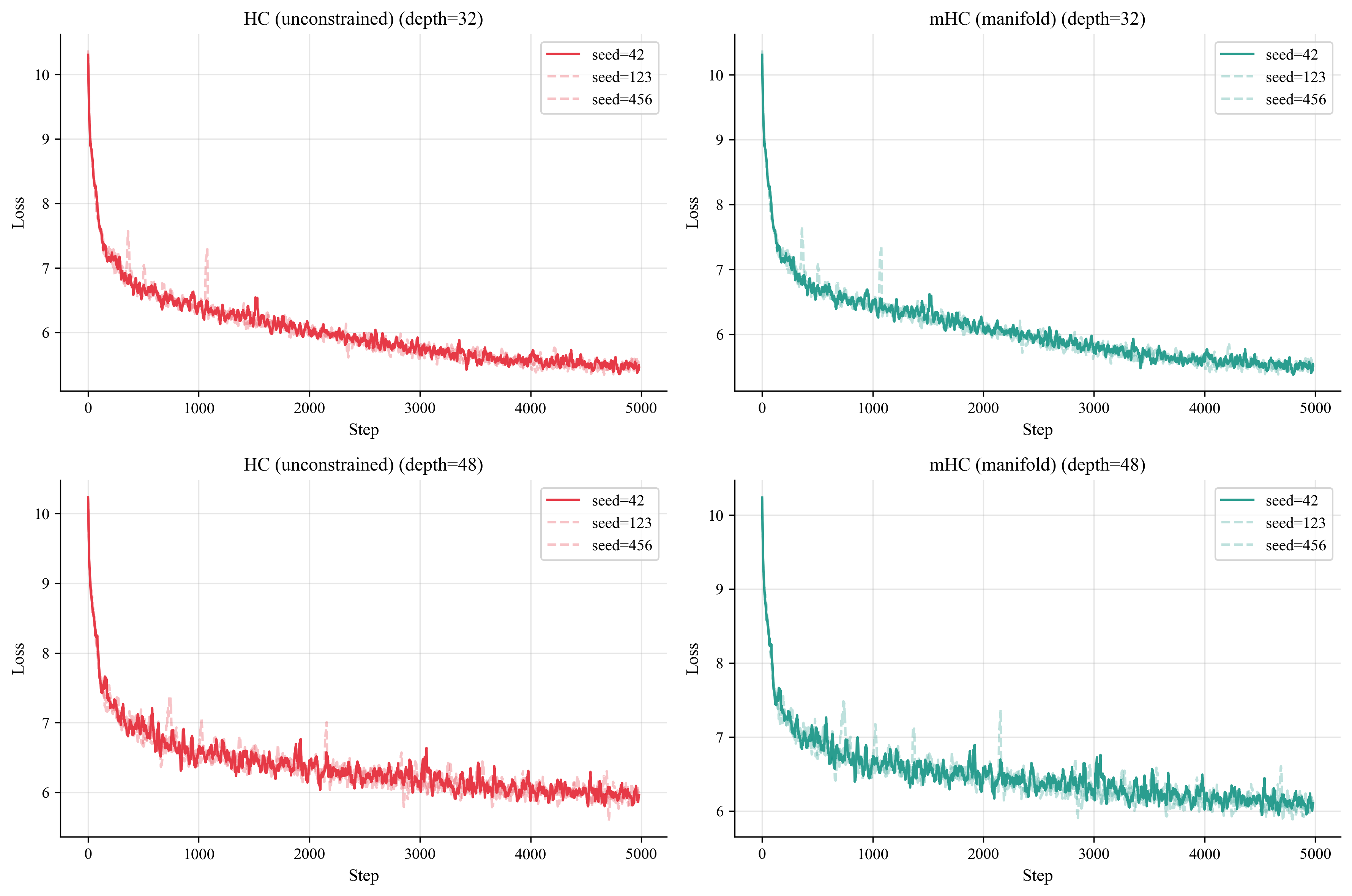
Loss and amplification curves for three seeds of each architecture. The loss curves lie on top of each other; every unconstrained amplification curve rises steeply and every constrained one stays flat. — *Fig. 4* The depth-32 runs broken out by seed (42, 123, 456), 5,000 steps each. Every unconstrained run diverges and every constrained run stays at 1.00, but the size of the divergence is highly seed-dependent: 6,545, 11,919 and 14,308 across the three. The loss curves overlap across all six. Colour separates the two arms and each is labelled; with three seeds the spread is reported as a standard deviation and nothing narrower is claimed. Runs runs_c4/hc_d32_s{42,123,456} and runs_c4/mhc_d32_s{42,123,456} .

Three seeds, one pattern: every HC run explodes and every mHC run stays flat, and the loss curves overlap across all of them. The only difference is inside the network.

Per layer: where the instability starts

Largest anywhere in this run: 1.9464866 at layer 0, step 2,830.

Largest anywhere in this run: 1.0000002 at layer 27, step 174.

2.0 is off the top of this scale — no layer of either run ever reaches it. The dark end is the largest cell drawn; each panel's own line below it gives that run's largest value over all 5,000 stored steps, which can be higher because the peak fell between two kept steps. Magnitude, not a verdict: the ramp is achromatic on purpose.

Fig. 5Per-layer amplification over training, unconstrained beside constrained, depth 32 seed 42. Layers run down each panel and sampled training steps across. This is a magnitude and not a verdict, so the scale is achromatic and shared between the panels: light is small, dark is large.

Every cell is one stored number: max(attn, ffn) for that layer at that step, read out of the run's history.json. Columns are stored steps — every 129th of 5,000, first and last kept — so no cell averages a range. Layer 0 is the top row of each panel.

The surprise here is that the instability starts at the input, not the output.

Layer 0 is where amplification appears first and stays largest. Across the three depth-32 seeds its mixing matrix peaks at 1.98, 1.95 and 1.93 while every deeper layer sits near 1.0, and layer 0 is the peak layer in 17 of the 19 unconstrained runs in this project that stored per-layer values. It does clear 2.0, but never at the 1e-4 learning rate these runs use: the five runs that pass it all trained at 3e-4 or above, topping out at 2.59. Depth doesn’t look like the problem. Layer 0 is, and it’s the only layer that sees the raw input.

Every deeper layer sits behind a LayerNorm and sees normalised representations. The first mixing matrix gets whatever the embedding table produces, and if the scale isn’t matched, it learns to compensate. In HC, compensating can mean amplifying.

mHC is uniform across every layer and every step, never leaving 1.0000 to four decimal places.

Signal flow

Fig. 6What a signal picks up walking layer 0 to layer 31 at training step 3,000, depth 32 seed 42: the running product of each layer's amplification. Purple and solid is the unconstrained arm, green and dashed the constrained one, both named on the figure.

HC, unconstrained — solid mHC, Sinkhorn-constrained — dashed

The running product of max(attn, ffn) taken in layer order at step 3,000. Ten of the 32 layers are marked; the end value is the product over all 32, so it is the run's real figure and not the product of the marks. HC ends at 532.391×, mHC at 1.0000029×.

At step 3000 a signal entering the HC network is 532× larger by the time it leaves. The same signal through mHC leaves at 1.000003×. LayerNorm and the non-linearities mop up a lot of that in HC, which means they’re spending capacity counteracting the mess upstream instead of doing anything useful.

The stress test

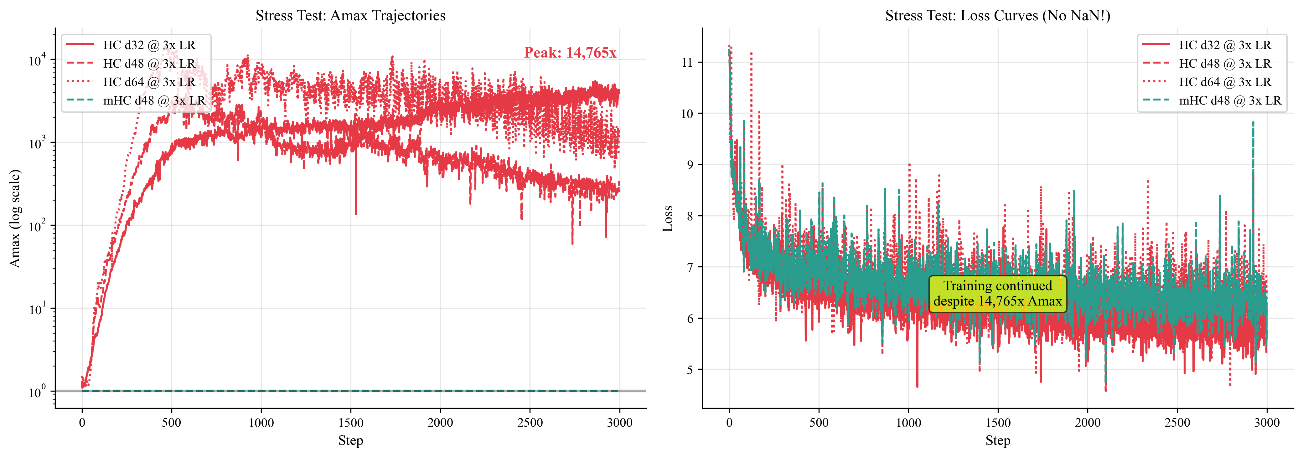
Peak amplification under a tripled learning rate at three depths, against the constrained arm which stays at 1.0 in every configuration. — *Fig. 7* The same architectures at three times the normal learning rate (3e-4 against 1e-4), one run per configuration. Unconstrained peaks: about 5,400 at depth 32, about 3,800 at depth 48, and 14,765 at depth 64, after which it oscillates between about 2,000 and 10,000. The constrained arm is 1.0 in every configuration and every learning rate tried. One seed per configuration, so the ordering between depths here is not separable from seed noise — Fig. 4 shows how wide that is.

Normal training used a learning rate of 1e-4. I also ran every configuration at three times that:

Config	Max Amax
HC d32 @ 3x LR	~5,400x
HC d48 @ 3x LR	~3,800x
HC d64 @ 3x LR	14,765x
mHC (all configs)	1.0

The depth-64 model hit 14,765× and then oscillated between about 2,000× and 10,000× for the rest of training. mHC was 1.0 at every depth and every learning rate.

Nothing crashed

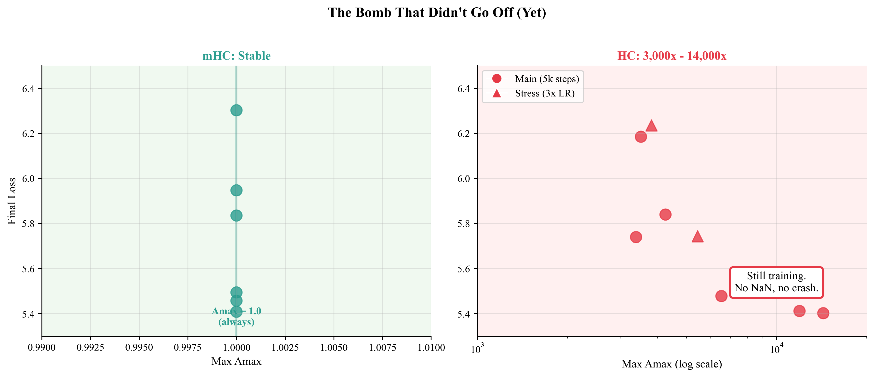
Panels showing large signal amplification alongside loss curves that keep descending smoothly and gradient norms pinned at the clipping threshold. — *Fig. 8* Amplification against training health for the same runs. None of the unconstrained runs diverged, went to NaN, or stopped learning, at up to 14,765× amplification. The gradient norm sits at the clipping threshold of 1.0 throughout, which is the most likely reason. This figure shows a co-occurrence over 5,000 steps and does not test whether the instability would eventually cause failure; that question is open and is stated as open in the text.

I didn’t expect this part: none of the HC runs crashed. At 14,765× and at 10,924×, loss didn’t diverge, nothing went to NaN, and the models kept learning. The gradient norm sits at the clipping threshold of 1.0 throughout, and clipping is almost certainly what held it together. Whether it would hold over more steps, or at 100B parameters, these runs can’t say. What they can say is that the amplification is there whether or not it has caused a failure yet, and that mHC doesn’t have it.

The conservation law, again

In Part 1, I framed residual connections as a conservation law:

Every residual connection is a conservation law. mHC enforces it.

At 1.7B that’s concrete: HC lets signals grow by 10,000× over training and mHC holds them at 1. At 10M, the 9.2× from Part 1 was manageable. At 1.7B a signal that should be magnitude 1 is magnitude 10,924, and the optimiser is doing extra work against the network’s own amplification the whole time. That’s at 5,000 steps. Longer training, a higher learning rate or a bigger model all push the same way. mHC doesn’t reduce the failure mode; it removes it.

What I learned running this

GPU 3 was dead. One of the 8 H100s kept throwing CUDA errors on a specific experiment. I wasted an hour debugging “code issues” before realizing it was hardware. Cloud GPUs fail.

Batch size constraints are real. The 2.5B parameter d48 models couldn’t fit at batch size 8. I had to drop to batch size 4. This means different tokens-per-step across depths. The HC vs mHC comparison at each depth is still valid (same batch size), but the cross-depth comparison is imperfect.

If you’re implementing Hyper-Connections

Use the Sinkhorn projection. It’s about ten lines and it removes the failure mode.
Monitor Amax during training. If you see it climbing past 10x, you’re building up instability.
Layer 0 is the canary. Watch your input mixing matrix especially closely. If your base model has an unstable Layer 0, vocabulary changes or embedding shifts during fine-tuning could destabilize the network.
The constraint cost nothing here. mHC matched HC loss in every run.

Code and data

The data and the code are public.

W&B (main experiments): wandb.ai/taylorkolasinski/mhc-part2
W&B (stress tests): wandb.ai/taylorkolasinski/mhc-part2-stress
Repository (training scripts): github.com/poisson-labs/mhc-repro

The W&B dashboards have full configs, metrics, and system logs for every run.

The experiments ran on a Lambda Labs 8x H100 SXM5 node: about thirteen hours of runs.

What’s next

Two open questions:

Does HC actually fail? I saw 10,924x amplification, but training didn’t diverge. Is this latent risk, or would longer training cause failure?
What’s the scaling law? 10M → 9.2x. 1.7B → 10,924x. What happens at 10B?

I want to run this at 10B, where the trend line says 50,000×. The experiment is ready to go and needs a step up in compute. If a GPU provider wants to back Part 3, my DMs are open.

In my setup this isn’t a theoretical issue. I can measure it, reproduce it, and it’s already about 10,000× past what I’d personally consider safe.

Questions or feedback: @TayKolasinski