Map the Failure Boundary

August 19, 2026

Software gets unit tests. Systems that learn, from RL policies to LLM agents, mostly get a benchmark score and a demo video, and a system that succeeded once tells you very little about how often it will succeed again.

We built Proofload to map where those systems fail, and the first thing we pointed it at was a trained Unitree Go1 locomotion policy: frozen, then run through 400 combinations of floor friction and lateral push, 16 times each, 6,400 rollouts in all. Each cell is a small experiment. Run the trials, record the time to failure, turn the outcomes into an estimate of surviving the five-second episode. The same setup lets us probe single worlds, look at the trajectories, and run the whole thing again after retraining.

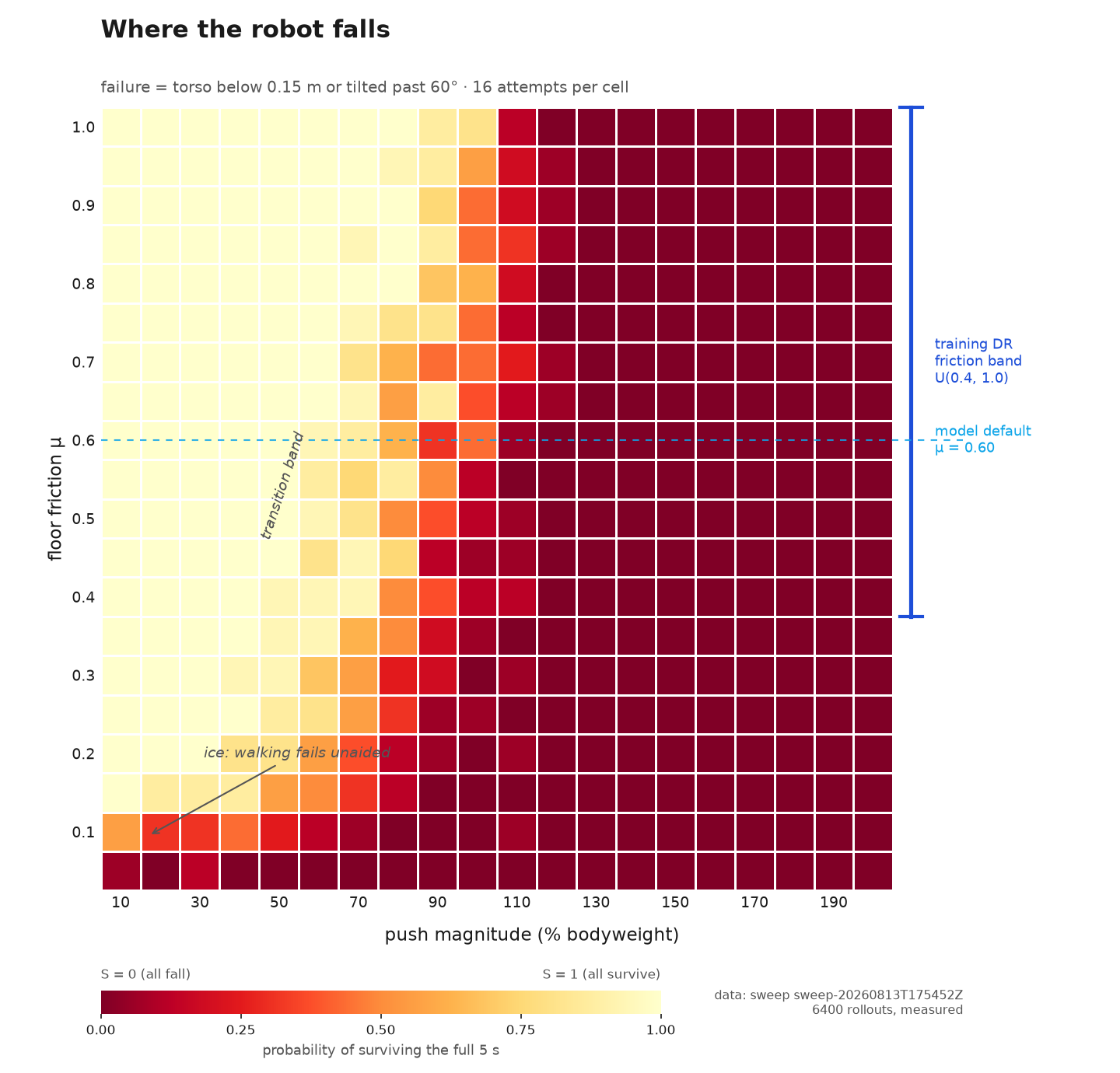
Kaplan-Meier survival surface: friction vs push magnitude, 400 cells — Survival probability across the grid. Pale cells survive the full 5-second episode; dark cells fall. Push magnitude runs left to right (10–200% of bodyweight); floor friction runs bottom to top (μ 0.05–1.00).

6,400 rollouts · 20×20 conditions · 16 trials per cell · 126 s of GPU time

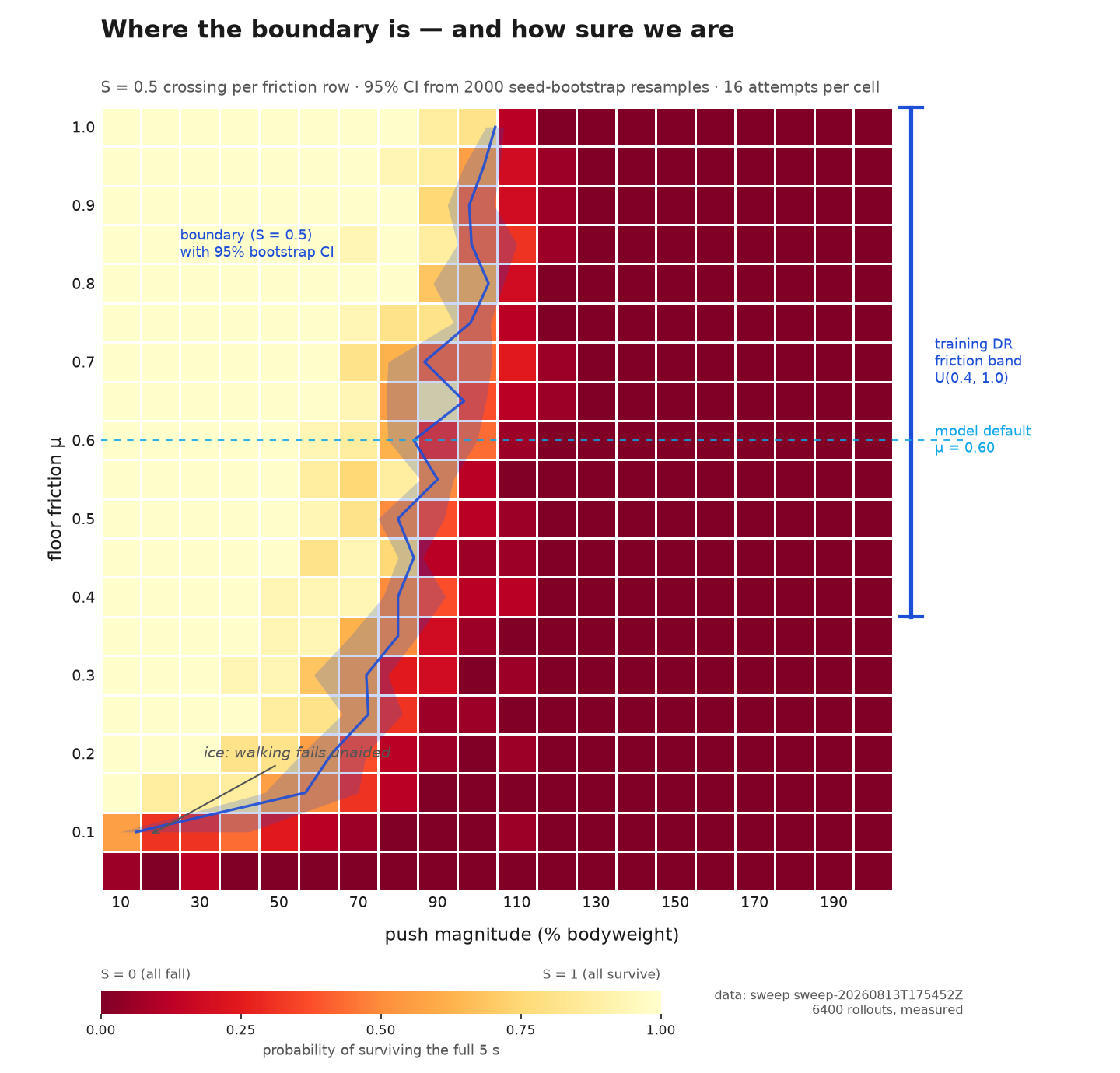
The sweep went into the store on the afternoon of August 13. It came back with a boundary that is a band rather than a threshold, ±4% of bodyweight on high friction and ±33% on ice, and a region below μ ≈ 0.15 where the policy falls before the push matters at all. After retraining on exactly the two things the map said training had missed, 60 cells were significantly safer and none were worse. The whole thing, retraining and the repeat sweep included, cost $42.

Nine worlds, one push, synchronized at t=2s. Friction increases bottom-to-top, push magnitude left-to-right.

The result

The boundary is diagonal: grippier floors tolerate harder pushes. On medium friction the policy survives pushes up to roughly its own bodyweight (about 125 N for this 12.7 kg robot) and fails beyond that. Before running anything we’d guessed the boundary near 15 N from a back-of-the-envelope estimate. The measured value is several times higher, which is one reason this post only reports numbers that were measured.

The failure we didn’t expect is at the bottom of the map. Below μ ≈ 0.15 it goes dark at the left edge: the robot falls at a 10% bodyweight nudge, or with no push at all. On ice the policy can barely walk. That’s a different failure from being knocked over (the gait itself collapses), and it lives entirely outside the friction range the policy trained on.

The boundary is also not a sharp threshold. Bootstrapping the 16 trials in each cell (2,000 resamples) gives a 95% interval on each row’s crossing point: about ±4% of bodyweight on high friction, ±33% on ice, a 7× spread. A single curve would hide that width, and the width is part of the finding.

Boundary as a 95% confidence ribbon per friction row — The S=0.5 crossing per friction row with its 95% bootstrap interval. Median width is about 16% of bodyweight; the boundary is sharpest where the policy is most comfortable.

Method

A demo video is one draw from a stochastic system and says little about the conditions next door. The grid is there to measure the distribution, which conditions the policy survives and how often, cheaply enough that we could measure it again after every training change.

Policy. Go1 joystick locomotion (MuJoCo Playground’s recipe, Brax PPO), trained once for 217.9M steps (736 seconds on one A100) to a nominal reward of 30.30 ± 0.54, then frozen.
Training distribution. Friction randomized over U(0.4, 1.0), with mass, center-of-mass, and joint jitter, and no pushes. Every push in this study is out-of-distribution by construction, and the bottom third of the friction axis is below anything the policy saw.
Perturbation. A constant lateral force on the torso for 0.5s, starting at t=2s, applied in physics only; the observation the policy sees is untouched. 100% of bodyweight = 125.0 N.
Failure. Torso below 0.15 m or tilt past 60°, whichever comes first, with thresholds frozen before the sweep. Rollouts that survive the 5-second window are censored, not counted as late failures. We use survival analysis (Kaplan–Meier per cell) precisely because some trials never fail.

One cell of the map, three camera angles: μ=0.35, an 80% bodyweight push at t=2s, time-to-failure 2.72s. The clip freezes at the failure moment: the training simulator models foot-ground contact only, so a fallen body has nothing to rest on.

Validating the measurement

Before trusting the map we tested the measurement itself, three ways, and the third changed how we keep results.

Harness fidelity. The evaluation harness reproduces the training environment: we verified that replaying the nominal trajectory through the injection path yields identical states over 500 steps, and that the push enters through physics only.

Numerical sensitivity. Halving the timestep moved the boundary within bootstrap noise; doubling solver iterations moved it by about 17% of bodyweight. That’s real, and reported, but small next to the structure. The diagonal band and the ice cliff persist under every solver setting we tried.

Nondeterminism. Repeated GPU runs of the same program and seed can diverge: floating-point reduction order is not fixed, and a thousand steps of contact dynamics amplify it. We report distributions, not individual trajectories. Some knife-edge survivors cannot be re-simulated. Their replay exists in the cache or not at all, which is why the first probe of each world is kept as its canonical record.

A knife-edge survivor: μ=0.80, a 100% bodyweight push, with minimum uprightness 0.66 and minimum torso height 0.148 m, both just above the failure thresholds. It recovers. The most dramatic recorded survivor at this cell could not be re-simulated; this is its nearest reproducible neighbor.

Intervention

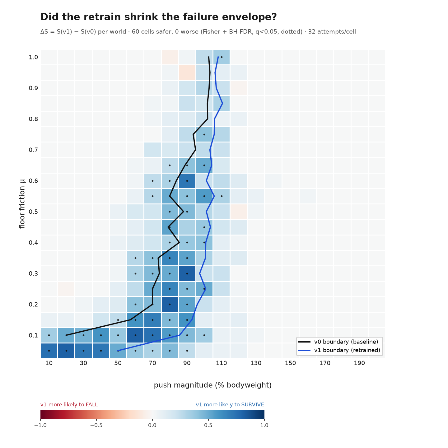
The map identified two conditions missing from training: the policy had never been pushed, and had never walked on friction below 0.4. We changed exactly those two settings (the environment’s own perturbation kicks, and a friction range widened to U(0.1, 1.0)), retrained with an otherwise identical recipe in about 12 minutes, and ran the same sweep again.

60 of the 400 cells became significantly safer (Fisher’s exact test with Benjamini–Hochberg correction across all cells, q < 0.05). None became significantly worse. The measured crossing (each row’s bootstrap-median boundary) moved outward on every friction row, most in the regions where training was widened: at μ=0.10 it rose by about 66% of bodyweight, and at μ=0.05, where the baseline couldn’t walk at all, the retrained policy has a boundary for the first time, with its survival crossing near a 50% bodyweight push. High-friction rows, already inside the original training distribution, moved only 4–8%.

v0 baseline

v1 retrained

The same world (μ=0.60, a 90% bodyweight push) measured on both policies: the baseline falls at 2.66s; the retrained policy staggers and recovers. Representative rollouts; seeds differ per side.

Difference surface: retrained policy minus baseline, per cell, with significance — Per-cell change in survival, retrained minus baseline. Blue = improvement; dots mark significance (Fisher + BH-FDR, q < 0.05). The retrained boundary (blue curve) sits outside the baseline (black) on every row.

Probe the map

The map is also interactive: pick a friction/push combination with the sliders and the corresponding rollout loads in the viewer. Worlds that have been probed before are cached and load instantly, at no cost; a new world runs a fresh rollout on a serverless A100 via Modal (about 3 seconds warm, ~25 seconds cold) and its first replay becomes the canonical record for that world.

floor friction μ 0.35 push 80% BW

loading viewer…

What it cost

All of the compute runs on Modal’s serverless A100s, scaled to zero between uses. A full 6,400-rollout sweep takes about 126 seconds; a fresh interactive probe is about 0.5 seconds of physics and 3 seconds end-to-end when warm.

Training: 736 seconds, once. Retrain + re-sweep + diff: about 14 minutes.
Idle, between probes: $0.
The full experiment, including retraining and the repeat sweep: $42, read off the bill rather than a rate card.

At that price it can run after every training change instead of once at the end.

Scope and limitations

This is a map of one policy’s failures inside the simulator it was trained in. It isn’t a claim about a physical Go1 on a physical floor: the boundary belongs to this policy and this simulator, and the ice regime in particular is far outside the training distribution. Reproducibility across hardware is statistical (the surface within tolerance), not bitwise, for the nondeterminism reasons above.

Summary

We started with a frozen policy, mapped where it failed, changed the two parts of training the map pointed at, and ran the same test again. The second surface improved where we expected it to.

The part worth keeping is the loop: sweep, look at the failures, retrain, sweep again, at a cost that makes it practical to repeat. The tooling is Proofload, and nothing in the loop is specific to a quadruped. It fits any learned system too stochastic for a single demonstration to say much about.

Built on MuJoCo Playground, MuJoCo Menagerie (Unitree Go1 model), Brax, Rerun, and Modal. The Go1 model and Playground recipe are used under their respective licenses.