Where V-JEPA 2.1's Dense Features Hold Up (and Where They Don't)

May 6, 2026

A pre-registered robustness study across all four V-JEPA 2.1 model sizes, with deployment lessons.

TL;DR

We pre-registered a robustness study on Meta’s V-JEPA 2.1 (released March 2026) and ran it across all four released model sizes, ranging from 80M to 2B parameters. Three findings from the 322-cell sweep stand out:

• V-JEPA 2.1’s dense features are partitioned. They predict downstream task failure under temporal corruption (frame drops, occlusion, r = 0.35–0.37), but are statistically indistinguishable from zero correlation under image-noise corruption (Gaussian, motion blur, low-light). Parametric robustness on one axis does not transfer to another.
• Bigger is not reliably better. Every Tier 1 perturbation tested showed non-monotonic robustness across the four model scales. The 2B “gigantic” model is actually less robust than the 1B “giant” variant on three of the five perturbations.
• V-JEPA 2.1 is meaningfully orientation-sensitive. A simple horizontal flip, which preserves all temporal structure, disrupts feature representations as severely as playing the video backwards.

Why this study matters in practice

This isn’t an academic exercise. Poisson Labs is integrating V-JEPA-family models as the perception backbone for two production robotics workloads:

• Industrial Cable Insertion: Manipulation policies for sub-millimeter industrial cable insertion in cluttered environments. Visual conditions vary wildly across lighting, self-occlusion from the manipulator, and frame-rate variability under network constraints.
• Drone Infrastructure Inspection: Autonomous flight perception for tower and pipeline inspection, where camera roll is constant during maneuvers, motion blur is a perpetual factor, and low-light operations are common.

The Appeal of JEPA as a World Model Backbone

V-JEPA 2.1 is positioned as a “world model,” a system with an internal representation of how the physical world functions. Unlike generative models that consume massive compute to reconstruct high-entropy pixels, the JEPA architecture predicts only in a compressed latent space. This offers two benefits for robotics:

• Focus on action over appearance. Generative pixel prediction asks “What does this look like?” JEPA latent prediction asks “What is happening here?” By ignoring irrelevant visual noise like subtle lighting shifts, the backbone can focus on the underlying physics and causal structure of the scene.
• Safe mental simulation. World models let a robot simulate “imagined” futures, testing what happens if it grabs an object from a specific angle before it actually moves. The system learns from thousands of imagined errors without risking real hardware.

SOTA accuracy on clean benchmarks like Something-Something-V2 (SSv2) is a necessary baseline, but it tells us nothing about the model’s failure surface. For a robot in a factory or a drone in the wind, the relevant questions are:

• Graceful vs. catastrophic degradation. Is a linearly degrading feature recoverable through downstream training, or is there a sharp cliff that renders the system brittle?
• Architectural narrative vs. reality. V-JEPA 2.1 is positioned as a temporally consistent video model. If features are more fragile under temporal corruption than image-noise, engineering decisions based on the “temporal” narrative will be wrong.
• The scaling shortcut. Does moving to the 2B model reliably buy us deployability? If scaling is non-monotonic, model selection must be empirical and per-application.

This study answers those questions for the V-JEPA 2.1 family.

Methodology

V-JEPA 2.1 (Mur-Labadia et al., 2026) introduces dense features through a Dense Predictive Loss, deep self-supervision, and modality-specific tokenizers. The encoder ingests video as 16-frame clips and groups consecutive frame pairs into single temporal tokens. The architecture calls this a tubelet size of 2. So a 16-frame clip becomes 8 temporal positions, each carrying a small bit of cross-frame averaging by construction. This matters later for understanding why image-noise hits harder than frame drops.

We evaluated all four released sizes: ViT-base (80M), ViT-large (300M), ViT-giant (1B), and ViT-gigantic (2B).

The setup

We ran nine controlled perturbations across ten strength levels (s ∈ [0.1, 1.0]) on 200 SSv2 validation clips to build the core robustness curves. We then measured functional tracking degradation on 30 DAVIS clips (five perturbations × five strengths × four models) to ground the representation drift in a real-world task.

The metric hierarchy

For each clip, the encoder produces a grid of patch-level feature vectors at every temporal position. The three metrics measure different ways those features can drift between a clean clip and its perturbed version.

M1 (frame fidelity): Average cosine distance between matched patches at the same (time, position) in clean vs. perturbed. In plain terms: “How much did each individual patch’s representation move?” Low means the encoder produced almost the same feature at that location; high means the patch was reinterpreted.

M2 (temporal consistency): Cosine distance between temporal-gradient vectors (the per-patch difference feature(t+1) - feature(t)). We compare these gradient vectors clean vs. perturbed and average. In plain terms: “How much did the model’s sense of motion at each location drift?” This is the primary probe for V-JEPA’s core architectural claim of temporal consistency, because it isolates change between frames from the absolute frame content.

M3 (functional utility): Patch correspondence on DAVIS. We track ground-truth object regions across frames using the model’s features as the matching signal. In plain terms: “If you tried to actually use these features to track an object through the corrupted clip, how badly would tracking degrade?” This is the only one of the three that measures a downstream task rather than internal feature stability.

We pre-registered six hypotheses with explicit numerical decision rules before launch. That ruled out post-hoc metric tuning.

On sample sizes and seeds

200 SSv2 clips per cell sits within the standard range for video benchmarks (MVBench, CVRR-ES use 200–240 instances per task) and is comfortable for the effect sizes we observed. Bootstrap 95% CIs on per-cell M2 means are uniformly small (median ±0.015, max ±0.025 across all 200 cells). The smallest cross-model jump in the scaling story below (occlusion, +0.017) is 5.7× its CI half-width, well above the 2× threshold separating signal from noise.

We use a single random seed per cell, which follows ImageNet-C precedent (Hendrycks & Dietterich, 2019) for apples-to-apples cross-model comparison. With n = 200 clips per cell, between-clip variance dominates within-cell perturbation-realization variance. Multi-seed runs would tighten error bars but, given the size of the observed effects, would not flip any of the six hypothesis verdicts.

Calibration: the metric works as predicted

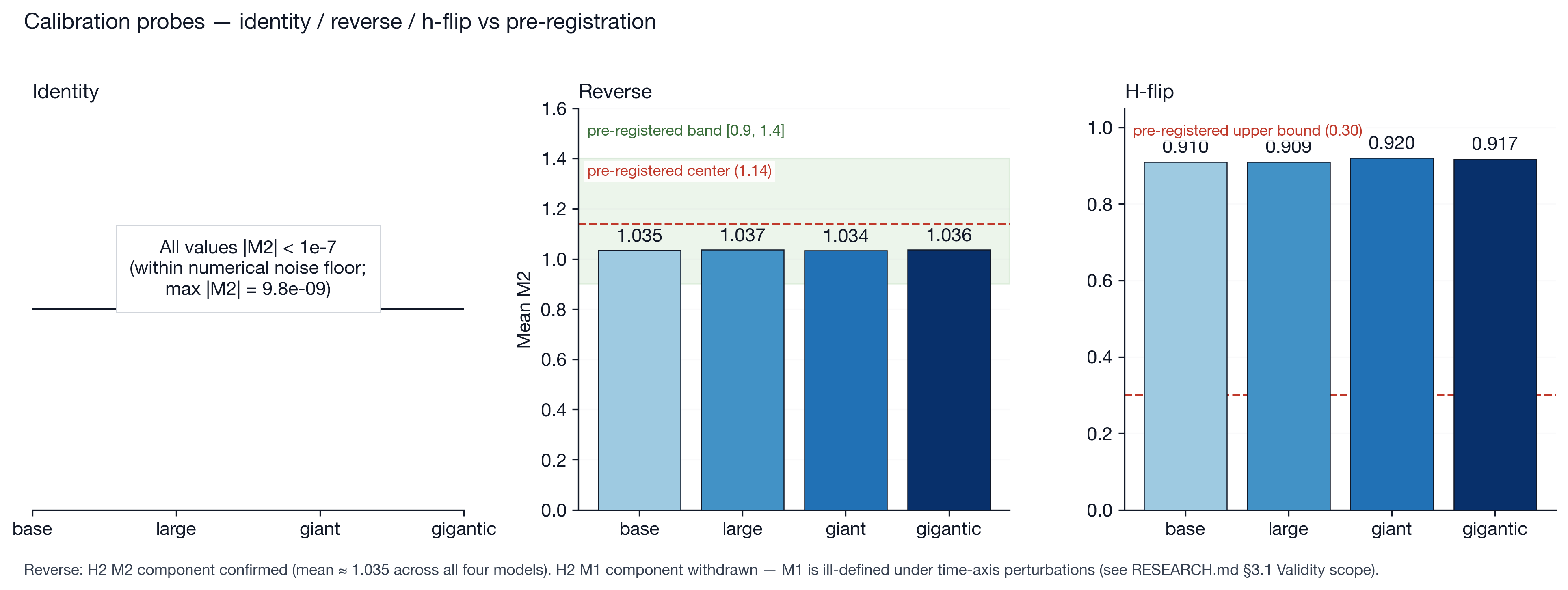
To validate the M2 metric, we derived an analytical prediction for its behavior under reverse-playback inputs: if you flip the clip so the last frame plays first, the temporal-gradient vectors should reverse direction, and (under a generic assumption that gradients are not pathologically aligned across frames) the cosine distance between clean-forward and perturbed-reverse gradients should land near a specific value. For a 16-frame input at tubelet size 2, that value is approximately 1.14.

Calibration on 30 DAVIS clips with ViT-base yielded mean M2 = 1.020 (std 0.036). Across the full SSv2 sweep, means for all four models clustered tightly between 1.034 and 1.037. Both numbers sit well within the predicted [0.9, 1.4] band. The DAVIS calibration (n = 30) and the SSv2 reverse cells (n = 200/model) have non-overlapping CIs but the gap is small and likely reflects DAVIS’s smaller, hand-curated clip distribution. The metric measures what the math says it should.

×

Finding 1: V-JEPA 2.1’s dense features are partitioned

The biggest finding: M2 (representational stability) only predicts downstream task failure (M3) for specific corruption classes.

The CIs for time-axis perturbations and image-noise perturbations do not overlap. The closest gap, between occlusion’s lower bound (+0.278) and motion blur’s upper bound (+0.171), is +0.106. The two perturbation families are statistically separable at 95% confidence. The aggregate r = 0.161 (95% CI [0.126, 0.195]) is distinguishable from zero but well below the pre-registered 0.30 ambiguous threshold and 0.50 confirmation threshold.

×

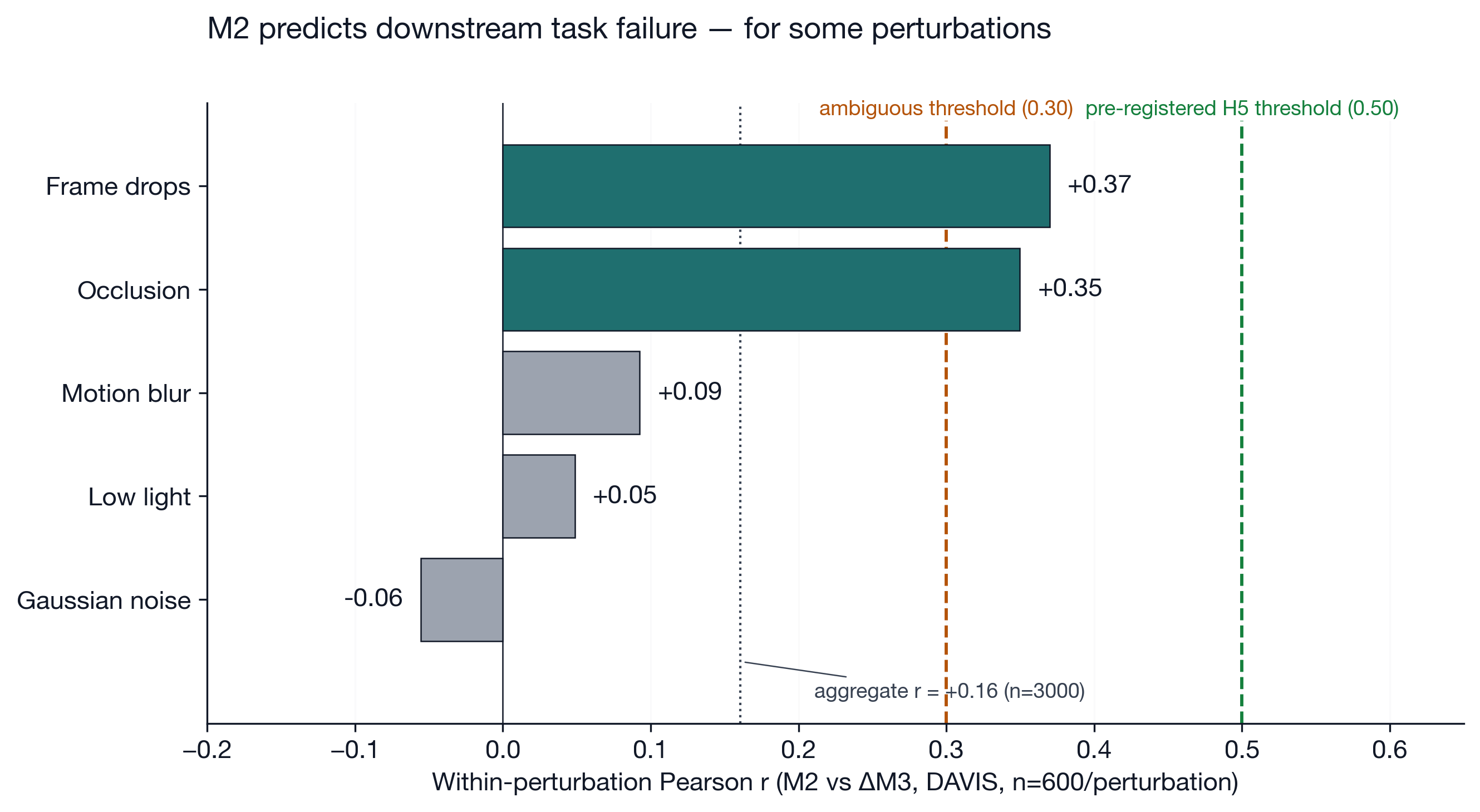
V-JEPA 2.1’s features appear to have two semi-independent axes: one image-content axis that is sensitive to noise but not load-bearing for tracking, and one temporal-structure axis that DAVIS-style correspondence depends on.

Deployment impact. For Cable Mind, where self-occlusion and variable frame rates are the primary stresses, M2 is a reliable health check. For Drone Inspection, where motion blur and sensor noise dominate, feature-level stability metrics will be misleading; we must use task-grounded evaluation instead.

Finding 2: Bigger is not reliably better

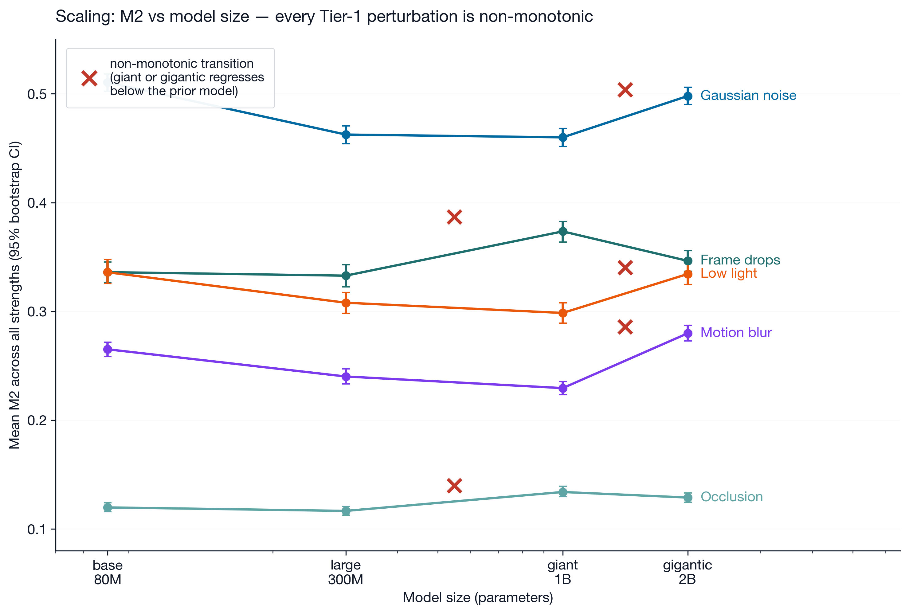
Contrary to monotonic scaling assumptions, robustness plateaus or reverses at the largest scales. In every Tier 1 perturbation, the scaling was non-monotonic:

• The 2B “gigantic” model was less robust than the 1B “giant” on Gaussian noise (+0.038 M2 jump), motion blur (+0.050), and low-light (+0.036).
• The 1B “giant” model was less robust than the 300M “large” variant on frame drops (+0.041) and occlusion (+0.017).

All five jumps clear at least 5× their pooled CI half-width. None are borderline noise.

×

One mechanistic explanation comes from recent work on what’s called hub marginalization in deep ViTs (arXiv:2511.21635). The short version: in a Vision Transformer, the special [CLS] token is supposed to act as a global summary, the place where information from every patch gets aggregated. As models get deeper and better-trained, that single hub becomes less load-bearing; the patch tokens themselves start carrying distributed information rather than routing everything through one summary node. This is generally good, until a model goes too deep and crosses into an “over-communication” regime where extra layers scramble information instead of refining it. V-JEPA 2.1’s training objective (the Dense Predictive Loss) explicitly pushes against single-hub aggregation by forcing every patch token to retain local identity. If the 2B variant has crossed into the over-communication regime while the distilled 300M variant retains controlled mixing, the non-monotonic robustness pattern is exactly what hub marginalization predicts. Distillation lineage is the second mechanism. The smaller variants are distilled from the 2B teacher per the released filename convention (*_dist_vitG_*), so they may inherit teacher-level robustness without the teacher’s full capacity costs.

Deployment impact. Scaling to 2B parameters is not a shortcut to reliability. For Cable Mind, which operates on edge-class hardware, the 300M “large” variant is frequently the better choice. It has superior robustness to temporal gaps at a fraction of the compute cost.

Finding 3: V-JEPA 2.1 is meaningfully orientation-sensitive

We hypothesized that a horizontal flip would preserve M2 consistency because flipping every frame the same way changes where things are in space but doesn’t change how they move between frames. The temporal-gradient field should be unchanged in its local structure, just mirrored. The data refuted this: mean M2 = 0.914 across all models, comparable to the disruption caused by playing the video backwards.

V-JEPA 2.1’s representations are sensitive to absolute spatial orientation. Flipping space changes the feature identity of every patch, which then warps the temporal-gradient field. In other words: the model is not learning rotation- or reflection-invariant representations out of the box. A patch on the left side of the frame produces a different feature than the same content rendered on the right side.

Deployment impact. For Drone Inspection, where camera roll varies during flight, we cannot rely on V-JEPA to handle the rotation for us. We need to rectify images to a canonical gravity-aligned orientation before they reach the encoder, or train downstream layers explicitly to absorb the orientation sensitivity.

Finding 4: Image-noise hits harder than temporal corruption

V-JEPA 2.1’s architectural framing emphasizes “temporal consistency.” But M2 is actually more disrupted by per-frame noise than by time-axis gaps. At strength 0.5, Gaussian noise (M2 = 0.499) is 1.54× more disruptive than frame drops (M2 = 0.324, 95% CI on the ratio [1.48, 1.60]). The dominance is not strength-specific. Gaussian dominates frame drops on at least 3 of 4 models at every one of the 10 strengths tested.

V-JEPA 2.1 looks more like a strong per-frame encoder with light temporal smoothing than a true temporal world model. The tubelet-size-2 design likely contributes: because consecutive frame pairs are pooled into a single temporal token, dropping one frame within a pair still leaves the other frame intact, and the resulting token degrades less than you’d expect. Per-frame noise, by contrast, corrupts both halves of every pair simultaneously. There’s no within-tubelet redundancy to fall back on.

What’s next

This study establishes the parametric baseline. In Part 2, we will replace these fixed perturbations with a learned adversary under our Monte banner. The goal is to see if a small network trained to maximize degradation can find failure modes (like specific texture-sticking points) that a grid sweep missed.

Reproducibility. Code, manifests, raw shards, and the analysis notebook at github.com/poisson-labs/vjepa-stress.

Acknowledgments

V-JEPA 2.1 from Meta FAIR. Methodology inspired by the ImageNet-C work of Hendrycks & Dietterich (2019). Pre-registration discipline modeled on practices from cognitive science. Compute provided by RunPod.